Penrose:
from mathematical notation to beautiful diagrams
by Katherine Ye1, Wode Ni1, Max Krieger1, Dor Ma'ayan1, 2, Jenna Wise1, Jonathan Aldrich1, Joshua Sunshine1, and Keenan Crane1
1Carnegie Mellon University, 2Technion
appearing in SIGGRAPH 2020
Paper
Talk
Teaser video
Abstract
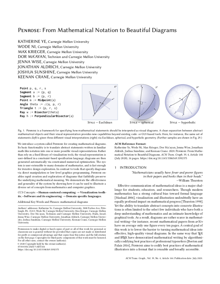
We introduce a system called Penrose for creating mathematical diagrams. Its basic functionality is to translate abstract statements written in familiar math-like notation into one or more possible visual representations. Rather than rely on a fixed library of visualization tools, the visual representation is user-defined in a constraint-based specification language; diagrams are then generated automatically via constrained numerical optimization. The system is user-extensible to many domains of mathematics, and is fast enough for iterative design exploration. In contrast to tools that specify diagrams via direct manipulation or low-level graphics programming, Penrose enables rapid creation and exploration of diagrams that faithfully preserve the underlying mathematical meaning. We demonstrate the effectiveness and generality of the system by showing how it can be used to illustrate a diverse set of concepts from mathematics and computer graphics.
Want to use Penrose or collaborate?
Please note that Penrose is an early-stage system that is still in development. Our system is not ready for contributions or public use yet, but we're working on it!
Want to be the first to hear about our system as we build it? Join our mailing list:
And reach out to us on Twitter: @UsePenrose
We're especially looking to talk with authors, educators, and expert illustrators who might be interested in collaborating on building a Penrose library for their area of expertise. Please fill out the form below (also accessible here) if interested.
Selected figures
Point p, q, r, s
Segment a := {p, q}
Segment b := {p, r}
Point m := Midpoint(a)
Angle theta := ∠(q, p, r)
Triangle t := {p, r, s}
Ray w := Bisector(theta)
Ray h := PerpendicularBisector(a)

Fig. 1. Penrose is a framework for specifying how mathematical statements should be interpreted as visual diagrams. A clean separation between abstract mathematical objects and their visual representation provides new capabilities beyond existing code- or GUI-based tools. Here, for instance, the same set of statements is given three different visual interpretations, via Euclidean, spherical, and hyperbolic geometry. (Further samples are shown in Fig. 29.)
PathType t
HasForm(t,"L(D|S)S*E")
Path p := Sample(t)
Fig. 4. By specifying diagrams in terms of abstract relationships rather than explicit graphical directives, they are easily adapted to a wide variety of use cases. Here we use identical Penrose code to generate ray tracing diagrams for several targets (Sec 5.6). Though the arrangement and number of objects changes in each example, the meaning remains the same.
For any vector space X, let u, v ∈ X be orthogonal vectors of equal length, and let w = u + v. Then u and w make a 45◦ angle.
VectorSpace X
Vector u, v ∈ X
Orthogonal(u, v)
EqualLength(u, v)
Vector w ∈ X
w := u + v

Fig. 7. Extensibility enables users to adopt conventions and notation that reflect the way they naturally write mathematical prose. Here, the resulting diagram plays the role of the concluding statement.
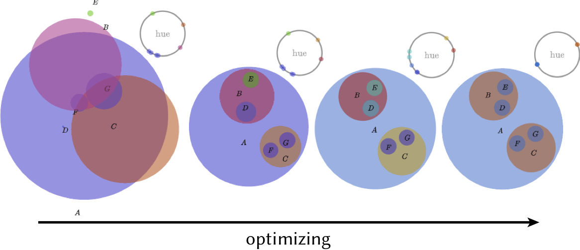
Fig. 8. An optimization-based approach makes it possible to jointly optimize visual attributes that are difficult to coordinate by hand. Here for instance we optimize color contrast according to the spatial proximity of adjacent disks (left to right), ultimately discovering a two-color solution (far right). The system can also be used to debug the optimization process itself—in this case by drawing the hue of each disk as a dot on a color wheel.

Fig. 9. A language-based design makes it easy to build tools on top of Penrose that provide additional power. Here we use standard techniques from program synthesis (Sec. 5.7) to automatically enumerate how the given relationships can be realized. Generating such examples helps to see important corner cases that might be missed when drawing diagrams by hand (where perhaps the top-left diagram most easily comes to mind).
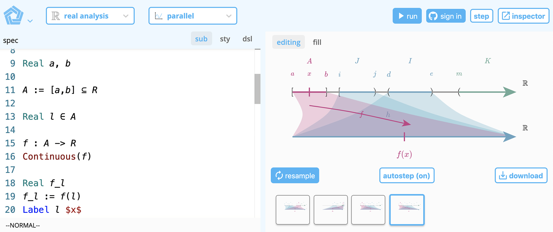
Fig. 17. Our system supports integration with web-based applications. Here a Penrose IDE provides automatic syntax highlighting and autocomplete for any user-defined domain.
-- Sets.dsl
type Set
predicate Intersecting : Set s1 * Set s2
predicate IsSubset : Set s1 * Set s2
predicate Not : Prop p
notation "A ⊂ B" ~ "IsSubset(A, B)"
notation "A ∩ B = ∅" ~ "Not(Intersecting(A, B))"
-- Sets.sub
Set A, B, C, D, E, F, G
B ⊂ A
C ⊂ A
D ⊂ B
E ⊂ B
F ⊂ C
G ⊂ C
E ∩ D = ∅
F ∩ G = ∅
B ∩ C = ∅
-- Sets-Disks.sty
forall Set x {
x.text = Text { string : x.label }
ensure contains(x.shape, x.text)
encourage sameCenter(x.text, x.shape)
layer x.shape below x.text
}
forall Set x; Set y
where IsSubset(x, y) {
ensure smallerThan(x.shape, y.shape)
ensure outsideOf(y.text, x.shape)
layer x.shape above y.shape
layer y.text below x.shape
}
forall Set x; Set y
where NotIntersecting(x, y) {
}

Fig. 18. Here, some Substance code is used to specify set relationships. Different Style programs not only tweak the visual style (e.g., flat vs. shaded disks), but allow one to use a completely different visual representation (e.g., a tree showing set inclusions). Sets.sty above describes the flat disk style.
-- Injection.sub
Set A, B
f: A -> B
Injection(f)
Not(Surjection(f))
-- Surjection.sub
Set A, B
f: A -> B
Surjection(f)
Not(Injection(f))
-- Bijection.sub
Set A, B
f: A -> B
Surjection(f)
Injection(f)
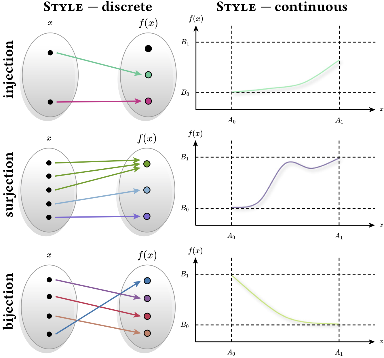
Fig. 19. Different visual representations provide different ways of thinking about an idea. Here, the notion of injections, bijections, and surjections is illustrated in both discrete (left) and continuous (right) styles. In the former, functions with the desired properties are randomly generated by an SMT solver, allowing the user to learn from many different examples.
Fig. 22. Once a complex diagram has been built, it can be easily broken into pieces or stages by, e.g., commenting out lines of Substance code. Here we illustrate steps in Euclid's proof of the Pythagorean theorem, turning Byrne's static figure (far right) into a progressive "comic strip."
SimplicialComplex K
Edge e ∈ K
Subcomplex E ⊆ K
E := Closure(e)
SimplicialSet StE ⊆ K
StE := Star(E)
Subcomplex ClStE ⊆ K
ClStE := Closure(StE)
Subcomplex ClE ⊆ K
ClE := Closure(E)
SimplicialSet StClE ⊆ K
StClE := Star(ClE)
SimplicialSet LkE ⊆ K
LkE := SetMinus(ClStE, StClE)

Fig. 24. A language-based specification makes it easy to visually inspect data structures or assemble progressive diagrams with only minor changes to program code. Here we draw the simplicial link by building it up from simpler constituent operations.
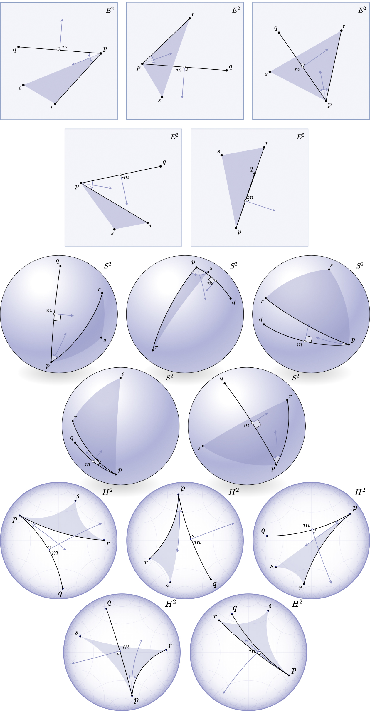
Fig. 29. Though the energy in the objective function can help guide a sampling strategy, choosing which diagram looks "best" to a given user is necessarily a subjective decision. The ability to automatically generate many alternatives makes it easier to find a satisfactory diagram. Here we show a gallery of automatically-generated variants of Fig. 1.
More information
-
Check out our CHI paper on natural diagramming!
Press
Acknowledgments
We thank Lily Shellhammer and Yumeng Du for their help. The first author was supported by a Microsoft Research PhD Fellowship and ARCS Foundation Fellowship while completing this work; the last author was supported by a Packard Fellowship. This material is based upon work supported by the National Science Foundation under grants DMS-1439786 and CCF-1910264, the AFRL and DARPA under agreement FA8750-16-2-0042, and the Alfred P. Sloan Foundation under award G-2019-11406.
How to cite
ACM reference format
Katherine Ye, Wode Ni, Max Krieger, Dor Ma’ayan, Jenna Wise, Jonathan Aldrich, Joshua Sunshine, and Keenan Crane. 2020. Penrose: From Mathematical Notation to Beautiful Diagrams. ACM Trans. Graph. 39, 4, Article 144 (July 2020), 16 pages. https://doi.org/10.1145/3386569.3392375
BibTeX
title = {Penrose: From Mathematical Notation to Beautiful Diagrams},
journal = {ACM Trans. Graph.},
volume = {39},
number = {4},
year = {2020},
publisher = {ACM},
address = {New York, NY, USA}
Project link